A Quantum Connection For Matrix Rank

Chaowen Guan is a PhD student at Buffalo. After a busy end to the Spring 2019 term at UB, we are getting time to write about our paper, “Stabilizer Circuits, Quadratic Forms, and Computing Matrix Rank.”

Today we emphasize new connections we have found between simulating special quantum circuits and computing matrix rank over the field .

The quantum circuits involved have been known as polynomial-time solvable since 1998. They are not universal but form important building blocks of quantum systems people intend to build. They impact the problem of showing quantum circuits are more powerful than classical circuits—the quantum advantage problem—in terms of how much harder quantum stuff must be added to them.

The question is: How efficiently can we simulate these special circuits? Our answer improves the bound from order- to , where here means the current best-known exponent for multiplying matrices (over or any field). Today stands at . The non-quantum problem of counting solutions to a quadratic polynomial modulo 2 is likewise improved from the shown by Andrzej Ehrenfeucht and Marek Karpinski to .

This comes at a price, however, because the matrix multiplication algorithms that optimize the exponent are galactic. In this post we’ll emphasize what is not galactic: reductions to and from the problem of computing matrix rank that run in linear time—meaning time for dense matrices—except for the need to check a yes/no condition in one of them. All this builds on the algebraic methods in our paper last year with Amlan Chakrabarti of the University of Calcutta.

Chaowen has contributed a post and some other materials for this blog. His work first came up in a post three years ago that saluted Dick and Kathryn’s wedding. Today is their third anniversary—so this post also comes with happy anniversary wishes.

Strong Simulation Problems

We have covered quantum algorithms several times. We discussed stabilizer circuits in an early post on the work with Amlan and covered them more recently in connection with the work of Jin-Yi Cai’s group. Suffice it to say that stabilizer circuits—which extend Clifford circuits by allowing intermediate measurement gates—form the most salient case that classical computers can simulate in polynomial time.

The simulation time is sometimes cited as going back to a 2004 paper by Scott Aaronson and Daniel Gottesman, but there is a catch: this is only for one measurement of one qubit. For general (non-sparse) instances, all of various other algorithms need order- time to re-organize their data structures after each single-qubit measurement. This is so even if one merely wants to measure all qubits in one shot: the time becomes . This is one case of what is generally called a strong simulation. It is precisely this time that Chaowen and I improved to .

In wider contexts, strong simulation of a quantum circuit means the ability to compute the probability of a given output to high precision. When the input and output are both in we may suppose both are since we can prepend and append gates to . Then strong simulation means computing the amplitude (or computing which is the output probability) to -place precision. It doesn’t take much for this to be -hard, often -complete. If we take the Clifford generating set

then we can get universal circuits by adding any any one of the following gates:

In the last one we’ve portrayed the matrix of the Toffoli gate as being block-diagonal. We will later consider block-diagonal matrices permuted so that all “blocks” are at upper left.

There is much recent literature on trying to simulate circuits with limited numbers of non-Clifford gates, and on how many such gates may be needed for exponential lower bounds—even just to tell whether . This plays against a wider context of efforts toward quantum advantage. Chaowen and I have been trying to apply algebraic-geometric techniques for new lower bounds at the high end, but this time we found new upper bounds at the low end.

From Matrix Rank to Quantum

It is not known how to compute the rank of a dense matrix in better than matrix-multiplication time, even over . We may suppose is square and symmetric, since we can always form the block matrix

and then 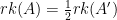. In the case of , is the adjacency matrix of an undirected bipartite graph . The rank of for any undirected graph must be even. Whereas the rank of the vertex-edge incidence matrix always equals minus the number of connected components of , less is known about characterizing . Our first main theorem brings quantum strong simulation into the picture. Let stand for .

Theorem 1 Given any we can construct in time a stabilizer circuit on qubits such that

One interpretation is that if you believe matrix rank is a “mildly hard” function (with regard to -time computability) then predicting the result of measuring all the qubits in a stabilizer circuit is also “mildly hard.” Such mild hardness would represent a gap between the time for weak simulation and the time for strong simulation. Such gaps have been noted and proved for extensions of stabilizer circuits but those are between “polynomial” and an intractable hardness notion.

One can also view Theorem 1 as a possible avenue toward computing matrix rank without doing either matrix multiplication or Gaussian elimination. This is the view Chaowen and I have had all along.

From Quantum to Rank

The distinguishing point of our converse reduction to the rank is knowledge of normal forms that depend on where one can use the knowledge to delay or avoid computing them explicitly. The normal forms are for polynomials associated to quantum circuits in our earlier work. Stabilizer circuits yield as a classical quadratic form over , the integers modulo . That is, all cross terms in have even coefficients—here, or . Thus quantum computing enters a debate that occupied Carl Gauss and others over two hundred years ago:

Should every homogeneous quadratic polynomial with integer coefficients be called a quadratic form, or only those whose cross terms all have even coefficients ?

The point of even coefficients is that they enable having a symmetric integer matrix such that

for all . Without that condition, might only be half-integral. This old difference turns out to mirror that between universal quantum computing and classical, because the non-Clifford -gate noted above yields circuits whose over have terms and/or . While counting solutions in for those polynomials is in , counting their binary solutions is -complete—an amazing dichotomy we expounded here.

We hasten to add that for the classical forms coincide with those over whose nonzero cross terms all have coefficient . Those are called affine in the work by Jin-Yi and others noted above, and our above-mentioned post noted his 2017 paper with Heng Guo and Tyson Williams giving another proof of polynomial-time simulation of stabilizer circuits via being affine. Our work improving the polynomial bounds, however, draws on a 2009 paper by Kai-Uwe Schmidt and further theory of classical quadratic forms. This paper uses work going back to 1938 that decomposes a classical (affine) quadratic form over further as

for binary arguments . Here is a binary vector with if or , otherwise, and the operations including the inner product are mod-2 except that the final is in . Then is alternating if the diagonal of is all-zero, non-alternating otherwise. Now take to be the rank of . The key normal-form lemma is:

Lemma 2 There is a change of basis to such that if is non-alternating then is transformed to

whereas if is alternating then is even and is transformed to

In either case, there is a binary vector so that for all .

The point is that to evaluate the quantum circuit , we don’t need to evaluate , but can make inferences about the structure of the solution sets to for , where . Given the knowledge of , the normal form goes a long way to this. The vector is also needed, but the fact of its having only bits gives hope of finding it in time. That—plus an analysis of the normal form itself of course—would complete an -time reduction from computing the amplitude to computing .

The Needed Piece—For Now

Chaowen took the lead all through the Fall 2018 term in trying multiple attacks. In the non-alternating case, the change of basis converts into a diagonal matrix over . In the alternating case, the same process makes a block-diagonal matrix of the kind we mentioned above. The conversion in both cases also yields . Of course can be computed by Gaussian elimination in time, but this is what we wanted to avoid.

After poring over older literature on -time methods, including a 1974 paper by James Bunch and John Hopcroft (see also this), we found a paper from last year by Jean-Guillaume Dumas and Clément Pernet that gives exactly what we needed: an LDU-type decomposition that yields in time. We only needed to apply the change-of-basis analysis in Schmidt’s paper to this decomposition and combine with the normal-form analysis to establish our algorithm for computing the amplitude :

1. Convert to the classical quadratic form with matrix over and associate the matrix over as above. This needs only time.

2. Compute the Dumas-Pernet decomposition 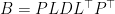over where is a permutation matrix, is lower-triangular, and is block-diagonal with blocks that are either or . Of course, this involves computing the rank of and takes time. Think of it as . This takes time—indeed, time according to Dumas and Pernet.

3. Compute over . This, too, takes time.

4. If any diagonal block of the original has become in , output . Else, is nonzero and we have enough information about and to find it—in only time, in fact.

This proves our main theorem:

Theorem 3 For stabilizer circuits , is computable in time. So is counting binary solutions to a classical quadratic form over , or any quadratic polynomial mod 2.

Because we use the decomposition, the above is not a clean -time reduction to computing . It does not make Theorem 3 into a linear-time equivalence. By further analysis, however, we show that the only impediment is needing in step 4 of our algorithm to tell whether . If we are promised that it is nonzero, then we obtain the probability in time from alone. This is actually where the power of Chaowen’s analysis of the normal forms is brightest and neatest. We will devote further posts to this and to illuminating further connections in graph and matroid theory.

A Three-Part Example

Consider the following quantum circuit . OK, this is a very low-tech drawing. Besides the six Hadamard gates it has two gates, which are shown as simple bars since they are symmetric:

By the rules given here, the three Hadamard gates at left introduce “nondeterministic variables” . The three Hadamard gates at right also give nondeterministic variables, but they are immediately equated to the output variables so we skip them. The polynomial is

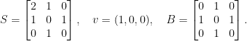
Upon substituting for all of and this gives simply . This is an alternating form with

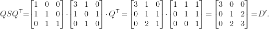
which is the adjacency matrix of the path graph of length 2 on vertices. Gaussian elimination does not need any prior swaps, so the permutation matrix in the decomposition is the identity and we get

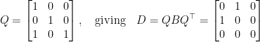
as the block-diagonal matrix over . Now we re-compute the products over to get

Now has entries that are but they are off-diagonal, and hence cancel when is computed in the -basis. Since is likewise the zero vector, this gives the transformed form as

It is easy to compute that has six values of 0 and two values of 2, which gives the amplitude as the difference divided by the square root of , so , The probability of getting as the result of the measurement is .

Now suppose we insert a -gate on the first qubit to make a new circuit . Since and are diagonal in the standard basis it does not matter where between the Hadamard gates it goes, say:

After substituting zeroes the form over is . This gives

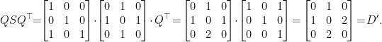
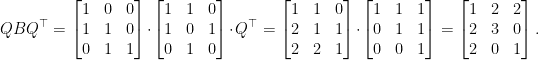
The matrix is the same as in the first example, hence so are the matrices and and the alternating status of . The difference made by and the resulting makes itself felt when we re-compute over :

Well, is far from diagonal—perhaps we shouldn’t use that name—but again the off-diagonal s are innocuous so we really have

The at upper left does not zero out the amplitude, because it is within a block. The at lower right, however, constitutes a block of , so it signifies that is not a possible measurement outcome. Essentially what has happened is that in the -basis the form has become

The isolated term in contributes mod to half the – assignments so as to cancel the other half, leaving a difference of in the numerator of the amplitude.

For the third example, let us insert a phase gate after the to make a circuit :

The combination is the same as , the adjoint (and inverse) of . Now after substitutions we have , giving:

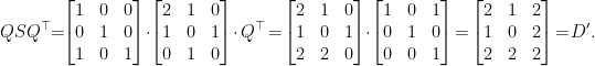
Note that is still a 0-1 matrix. This has full rank. Again it helps our exposition that is diagonalizable without swaps (and that the inverse of an invertible lower-triangular matrix is lower-triangular), so we can find with

In the -basis we get for some . To test for zero amplitude—before we know what is—we compute in :

Again we can ignore the off-diagonal ‘s. There is no on the main diagonal, so we know the amplitude is non-zero. To compute it, we only need the information on the diagonal, which tells us and in the transformed basis. Note that we could have written down the moment we learned that has rank over , so is the only rigmarole. The final analysis—using a recursion detailed in the appendix of our paper—gives the amplitude as

and so the probability of the output is .

We remark finally that is generally not the same as . To see where it comes from, let us now compute (not ) over to get . Then

where . Now off-diagonal elements in will cancel when taking modulo 4, so we need only retain the diagonal of as a binary vector. Since is binary, . This finally gives

with . In the third example we have and

The diagonal gives and so . This agrees with what we read off above by comparing with . There is a different worked-out example for the triangle graph on three vertices in the paper.

Looking Ahead

Chaowen and I continue to be interested in shortcuts to computing the amplitude and/or probability. Here we take a cue from how Volker Strassen titled his famous 1969 paper on matrix multiplication:

“Gaussian Elimination is not Optimal.”

We would like to find cases where we can say, “Matrix Multiplication is not Optimal.” In view of recent papers blunting efforts to show —see this post—the question may shift to which computations may not need the full power of matrix multiplication and be achievable in time after all. This applies to computing the rank (over ) itself, and the question extends to sparse cases like those considered in the paper, “Fast Matrix Rank Algorithms and Applications,” by Ho Yee Cheung, Tsz Chiu Kwok, and Lap Chi Lau.

The second circuit in the above example corresponds to a graph with a self-loop at node 1—or, depending on how one counts incidence of self-loops in undirected graphs, one could call it a double self-loop. It exemplifies circuits used to create quantum graph states, and those circuits are representative of stabilizer circuits in general. The third circuit can be said to have a “triple loop,” or maybe better, a “3/2-loop”—while if the original -gate were a single -gate giving the form , we would face the ambiguity of calling it a “loop” or a “half-loop.” Sorting this out properly needs going beyond graph theory. In upcoming posts, Chaowen and I will say more about how all this yields new problems in graph theory and new connections between quantum computing and matroid theory.

Open Problems

What do our results say about the problem of computing the rank of a matrix, and possibly separating it from dependence on matrix multiplication?

We hope that we have begun to convey how our paper uncovers a lot of fun computational mathematics. We are grateful for communications from people we’ve approached (some acknowledged in our paper) about possible known connections, but there may be more we don’t know. Our next posts will say more about combinatorial aspects of quantum circuits.

[fixed name]