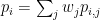
Depth of Satisficing

Tamal Biswas has been my graduate partner on my research model of decision-making at chess for over four years. He has I believe solved the puzzle of how best to incorporate depth into the model. This connects to ideas of the inherent difficulty of decisions, levels of thinking, and stopping rules by which to convert thought into action.

Today I describe his work on the model and the surprise of being able to distinguish skill solely on cases where people make mistakes. This is shown in two neat animations, one using data from the Stockfish 6 chess program, the other with the Komodo 9 program, whose elements are explained below.

Tamal presented this work on the Doctoral Consortium day of the 2015 Algorithmic Decision Theory conference in Lexington, Kentucky. The conference was organized and hosted by Judy Goldsmith, whom I have known since our undergraduate days at Princeton. The consortium was organized by Esra Erdem and Nick Mattei jointly with the co-located LPNMR conference. Our full paper, “Measuring Level-K Reasoning, Satisficing, and Human Error in Game-Play Data,” will be presented at the 2015 IEEE Conference on Machine Learning and its Applications in Miami. Tamal presented our predecessor paper, “Quantifying Depth and Complexity of Thinking and Knowledge,” at the 2015 International Conference on Agents and AI in Lisbon last January.

Although we have blogged about the chess research several times before, I haven’t yet described details of my model here. After doing so we’ll see why depth has been tricky to incorporate and what our new discoveries mean.

The Data

The only connection to chess is that chess has alternating turns involving decisions whose options can be given numerical utility values that are objective and reliable but difficult for the players to discern. The numbers come from powerful chess programs (commonly called engines) whose rated playing skill long surpasses that of human players and is arguably measurably close to perfection. The Elo rating system is scaled so that a difference of 100 rating points derives from and predicts a 64%-to-36% points margin for the stronger player. The World Chess Federation lists over 20,000 human players above the 2200 threshold for “master” but only 45 players above 2700 and just four above 2800 including world champion Magnus Carlsen at 2850—while the best engines are rated above 3200 and my model currently suggests a ceiling below 3500.

The move values are updated by the program in rounds of increasing search depth often reaching and beyond, by which they have most often stabilized. The highest option—or the first listed move in case of tied values—is the engine’s best move in the search, and its final value is the overall position value.

The numbers come from chess factors—beginning with basic values for the pieces such as pawn = 1, knight = 3, and so on—but they are governed by a powerful regularity. Position values are centered on 0.00 meaning “even chances,” positive for advantage to the side to move, and negative for disadvantage. The regularity is that when the average score (counting 1 per win and 0.5 per draw) achieved by players from positions of value is plotted against , the result is almost perfectly a logistic curve

The factor offsets the scale of the engine’s evaluation function—for a simple instance, whether it counts a queen as 9 or 10. Curiously the curve flattens only a little for two players of lower Elo rating. When there is a substantial difference in rating between two players, however, it does a strong horizontal shift:

A 2012 paper by Amir Ban not only observes this relationship (also separating out wins and draws) but argues that generating evaluations within the search that follow it optimizes the strength of the engine. We henceforth argue that the utility values have organic import beyond chess, and that the problem addressed by our model is a general one of “converting utilities into probabilities.”

By the way: Ban is famous for being a co-creator of both the Deep Junior chess program and the USB flash drive. That is right: the flash drive that we all use, every day, to store and transfer information—probably a bit more impactful than anything to do with chess, but amazing that he did both.

The Model and Depth

The model uses the move values together with parameters denoting skills of the player to generate probabilities for each legal move . Up to now I’ve used two parameters called for sensitivity and for consistency. They govern a term

where is a scaling adjustment on the raw difference . Lower and higher both reduce and ultimately the probability of an inferior move.

Chess has a broad divide between “positional” and “tactical” skill. I’ve regarded as measuring positional skill via the ability to discern small differences in value between moves, and as avoidance of large errors which crop up most often in tactical games. Neither uses any chess-specific features. Without introducing any dependence on chess, I’ve desired to enrich the model with other player parameters. Chief among them has been modeling depth of thinking but it is tricky.

My first idea was to model depth as a random variable with a player-specific distribution. As a player I’ve had the experience of sometimes not seeing two moves ahead and other times seeing “everything.” A discrete distribution specified by a mean for a player’s “habitual depth” and a shape parameter seemed to fit the bill. The basic idea was to use the engine’s values for at all depths up to the limit depth of the search in an expression of the form

A related idea was to compute probabilities from the values at each depth and finally set .

Doing so changed the regression from one over to one over and possibly . Whereas the former almost always has one clear minimum, the latter proved to be pockmarked with local minima having no global drift we could discern. Indeed, for many initial points, would drift toward with wild and values regardless of the skill of the games being analyzed. Perhaps this was caused by noisy values at the very lowest depths giving a good random match. I stayed with the two-parameter model in my official use and followed other priorities.

The Depth is in the Data

Looking back, I think my idea was wrong because depth is not primarily a human property. We don’t first (randomly) choose each time whether to be deep or shallow—to be a Fischer or a “fish” for a move. Instead, aspects of the position influence how deep we go before being satisfied enough to stop. One aspect which I had conceived within my scheme involves moves whose values swing as the depth increases.

A move involving a sacrifice might look poor until quite far into the search, and then “swing up” to become the best move when its latent value emerges. A “trap” set by the opponent might look tempting enough to be valued best at first even by the engines, but they will eventually “swing down” the value as the point of the trap is plumbed. The sublime trap that did much to win the 2008 world championship match for Viswanathan Anand over Vladimir Kramnik shows both phenomena:

Left: Position before Kramnik’s 29.Nxd4. Right: Anand’s winning 34…Ne3! riposte. Below: Stockfish 6 values x100 at depths 1–19.

Kramnik’s 29.Nxd4 capture might be dismissed by a beginner since Black’s queen can just take the knight, but a seasoned player will see the followup 30.Rd1 skewering Black’s queen and knight on d7. Evidently this looked good to Kramnik through 30…Nf6 31.Rxd4 Nxg4 32.Rd7+ Kf6 33.Rxb7 Rc1+ 34.Bf1 coming out a pawn ahead, and Stockfish turns from negative to positive throughout depths 9–14. But then it sees the shocking 34…Ne3!!, when after 35.fxe3 fxe3 Black’s passed pawn is unstoppable. Kramnik never saw these moves coming and resigned then and there.

In my old view, Kramnik pulled a number between 9 and 14 out of his thinking cap and paid the piper to Anand who had rolled 16 or higher at his previous turn. Based on the good fits to my two-parameter model, the reality that most positions are clear-cut enough even for beginners to find the best move over 40% of the time, and reasoning about randomness, I pegged the phenomenon as secondary and likely offset by cases where the played move “swung up.”

In Tamal’s view the whole plateau of 9–14 put friction on Kramnik’s search. Once Kramnik was satisfied the advantage was holding, he stopped and played the fateful capture. Of various ways to quantify “swing,” Tamal chose one that emphasizes plateaus. Then he showed larger effects than I ever expected. Between the 0.0–1.0 and 4.0–5.0 ranges of “swing up” for the best move in his measure, the frequency of 2700-level players finding it plummets from 70% to 30%. This cannot be ignored.

Depth of Satisficing

This result presaged the effectiveness of several other measures formulated in our ICAART 2015 paper to represent the complexity and difficulty of a decision. We introduced some ideas relating to test-taking in an earlier post but now we’ve settled on metrics. The most distinctive of Tamal’s ideas blends our investigation of depth with Herbert Simon’s notion of satisficing going back to the years after World War II.

Simon coined satisficing from “satisfy” and “suffice” and contrasted it to optimizing during a search. It is often treated as a decision policy of meeting needs and constraints, but Simon also had in mind the kind of limitation from bounded rationality (another term he coined) that arises in searches when information is hard to find and values are hard to discern. In a zero-sum setting like chess, except for cases where one is so far ahead that safety trumps maximizing, any return short of optimum indicates an objective mistake. We address why players stop thinking when their move is (or is not) a mistake. We use the search depth to indicate both time and effectiveness, gauging the latter by comparing the values given by the engine at depth and at the supreme depth .

Not all inferior moves have negative swing—their inferiority might lessen with —and not all moves of negative swing were valued best at some lower depths. For those that were valued best we can identify the depth at which the move is exposed as an error by the engine: in our example above. We judge that the player failed to look deeper than and call the depth of satisficing for that move.

We can extend the notion to include the many negative-swing cases where the played move does not actually cross with the ultimate best move . For each , plot the average over selected positions of and (note by definition, but if some other move is better at depth ). Over all positions the curves tend to be relatively close at low depths, but over positions with played move of positive swing the curve for stays significantly apart from that for , roughly paralleling it. This explains our persistent observation at all skill levels that over the negative-swing moves the curves do cross at some depth . Indeed, figures in our paper show that (green line below) is often significantly inferior to (red) at low depths. The crossover depth of the averages becomes the depth of satisficing for the aggregate.

Using UB’s Center for Computational Research (CCR) to run the engines Stockfish 6 and Komodo 9, we have analyzed every published game played in 2010–2014 in which both players were within 10 Elo points of a century or half-century mark (widened to 15 or 20 for Elo 1300 to 1650, 2750, and 2800 to keep up the sample size). Combining Elo 1300 and 1350, 1400 and 1450, etc., shows that the crossover depth grows steadily with rating in both the GIF for Stockfish (left) and the GIF for Komodo (right).

There we have it: a strong correlate of skill derived only from moves where players erred. The inference is that better players make mistakes whose flaws require more time and depth to expose, as measured objectively by the engines. A further surprise is that the satisficing depths go clear down near zero for novice players—that we got anything regular from values at depths below 4 (which many engines omit) is noteworthy. That the best players’ figures barely poke above depth 10—which computers reach in milliseconds—is also sobering.

Depth and Time

Chess is played with a time budget, much as one has when taking a standardized test. The first budget is almost always for turns 1–40, and although exhausting it before move 40 loses the game immediately, players often use the bulk of it by move 30 or even 25. The following moves are then played under “time pressure.” Segregating turns 9–25 from 26–40 (the opening turns 1–8 are skipped in the analysis) shows a clear effect of free time enhancing the depth and time pressure lowering it:

All of these games—this data set has over 1.08 million analyzed moves from over 17,500 games—come from recent real competitions, no simulations or subject waivers needed, in which skill levels are reliably known via the Elo system. Data this large, in a model that promotes theoretical formulations for practical phenomena, should provide a good standard of comparison for other applications. Tamal and I have many further ideas to pursue.

Open Problems

What parallels do you see between the thought processes revealed in chess and decision behaviors in other walks of life?

[added note on consortium organizers to intro, fixed Nxe3 in caption to Ne3]